Background

If you may remember, I concluded my last post with an outlook on learning unitary matrices with qgrad. This post goes into the details of what unitary learning is and how one can implement unitary learning in qgrad.

Unitary transformations are utterly important in quantum computing primarily because they preserve the norm of the vectors and thus keep the quantum states normalized. Quantum Machine Learning primarily intends to find a unitary transformation such that when a data vector, encoded as a quantum state, say $| \psi_{i} \rangle$, undergoes this transformation to give $U | \psi_{i} \rangle $, one can measure this state (in any particular basis depending on the problem) to evaluate the probability of an input vector belonging to a particular class in a classification task. Thus, efficient learning of unitary matrices is very useful in Quantum Machine Learning. Applications of learning unitaries are also widespread in the field of quantum control. Given its widespread applicability, we felt the need that qgrad users should be able to perform unitary learning routines smoothly with the library.

What is Unitary Learning?

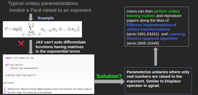
Suppose that I have a matrix $U$, and I want to learn $U(\theta)$, such that the entries of both $U$ and $U(\theta)$ are very close to each other, up to an irrelevant global phase. For a general matrix (which might not be unitary), you would need to find a parametrized factorization such that you can tune the parameters to get every entry of $U(\theta)$ as close as possible to every entry of $U$, again up to an irrelevant global phase. Thankfully for unitary matrices, many such parameterizations exist, as I detailed in my previous blog. Typically, these parameterizations involve a hermitian matrix in the power of the exponential, which is currently not differentiable in JAX. Following is the summary of the problem:

Parametrized Unitaries in qgrad

For those of you who read my last blog might recall that I was looking into different unitary parameterizations to select the one that would form qgrad’s backend for parameterized unitaries. Well, here it is. I implemented a scheme from Li Jing et al. (2017), where exponents only have real numbers in their powers – differentiable in JAX. On a side note, Li Jing et al. (2017) is a very interesting paper that uses unitary matrices to avoid vanishing/exploding gradients in classical neural nets. One may call this ‘quantum inspired’, but this was before QNNs were a thing. Anyway, back to the parameterization. $N$- dimensional parameterized unitary is defined as follows:

$$ \begin{equation}\label{unitary-param} U_{N} = D\prod_{i=2}^{N}\prod_{j=1}^{i-1}R^{’}_{ij} \end{equation} $$

where $D$ is a diagonal matrix, whose diagonal elements are $e^{i\omega_{j}}$ and $R_{ij}^{’}$ are rotation matrices where $R_{ij}$ is an $N$- dimensional identity matrix with the elements $R_{ii}, R_{ij}, R_{ji}$ and $R_{jj}$ replaced as follows:

$$ \begin{equation}\label{rot-matrices} \begin{pmatrix} R_{ii} & R_{ij} \\ R_{ji} & R_{jj} \end{pmatrix} = \begin{pmatrix} e^{i\phi_{ij}}cos(\theta_{ij}) & -e^{i\phi_{ij}}sin(\theta_{ij}) \\ sin(\theta_{ij}) & cos(\theta_{ij}) \end{pmatrix} \end{equation} $$

where $R_{ij}^{’} = R(-\theta_{ij}, -\phi_{ij})$ and $\phi_{ij}$, $\theta_{ij}$ and $\omega_{j}$ parameters are all real, which is what we desired (for compatibility with JAX).

Learning Unitaries with qgrad

Let us see how we can use qgrad to implement unitary learning routines. Here we will implement Seth Lloyd and Reevu Maity (2019) and the companion paper Bobak et al. In our implementation of these two papers with qgrad, we cheat a little bit, in that our unitary parameterization (\ref{unitary-param}) is different from that used by the authors

$$ \begin{equation}\label{decomp} U(\vec{t}, \vec{\tau}) = e^{-iB\tau_{N}}e^{-iAt_{N}} … e^{-iB\tau_{1}}e^{-iAt_{1}} \end{equation} $$

where $\vec{t}$ and $\vec{\tau}$ are parameter vectors of size $N$ and matrices $A$ and $B$ are chosen from a Gaussian Unitary Ensemble (GUE).

Fret not! You can see for yourself that parameterization (\ref{unitary-param}) implemented in qgrad has $\frac{N (N - 1)}{2}$ different $\theta_{ij}$ and $\phi_{ij}$ parameters and $N$ different $\omega_{j}$ parameters. Thus, the total number of parameters to approximate any unitary using this scheme scales as $O(N^2)$, where $N$ is the dimension of the unitary. The authors in Seth Lloyd and Reevu Maity (2019) conclude that an efficient reconstruction of a unitary takes $O(N^2)$ parameters. So, we don’t lose much with our new parametrization unless we want to reduce the number of parameters and end up with an inefficient reconstruction.

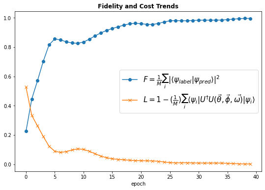
Alright, so for a target unitary matrix, $U$, the goal is to find optimal parameter vectors for the parametrized unitary $U(\vec{\theta}, \vec{\phi}, \vec{\omega})$, such that $U(\vec{\theta}, \vec{\phi}, \vec{\omega})$ approximates $U$ as closely as possible. For the purposes of this example, we work with $8$-dimensional (3 qubit) unitary matrices. Our the input dataset consists of $8 \times 1$ kets, call them $| \psi_{i} \rangle$ and output dataset is the action of the target unitary $U$ on these kets, $U |\psi_{i} \rangle$. The maximum value of $i$, which is equal to $M$, is $80$, meaning that we merely use 80 data points (kets in this case) to efficiently learn the target unitary, $U$. We use the same loss function as the authors of Seth Lloyd and Reevu Maity (2019) use in the original paper

$$ \begin{equation} \label{err_ps} E = 1 - (\frac{1}{M})\sum_{i} \langle \psi_{i}|U^{\dagger} U(\vec{\theta}, \vec{\phi}, \vec{\omega})|\psi_{i}\rangle \end{equation} $$

where $ |\psi_{i} \rangle$ are the training data points – in this case, kets, $U$ and $U(\vec{\theta}, \vec{\phi}, \vec{\omega})$ are the target and parameterized unitaries respectively, and $M$ is the total number of points in the dataset. In qgrad, this cost would look like

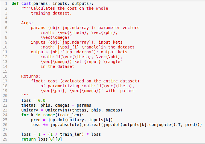
where one can parameterize unitaries by importing a Unitary class and calling the class object by passing parameters to it as is done in line 17 above. This parametrization in qgrad lets you differentiate the cost function in just one line using JAX’s grad. Speaking of learning, after a simple $40$ gradient descent steps, we match the input kets with the output kets with an average fidelity of $99.57 \%$.

Unitary Learning without qgrad

I made a separate tutorial without JAX and qgrad to juxtapose the convenience with which qgrad lets you differentiate functions. Without autodiff, there are two ways out. First is to write your own analytic derivative routines which can be very simple to very complex, depending on the function itself. For our cost function \ref{err_ps}, the derivative w.r.t $\tau_{k}$ would look like

$$ \begin{equation} \frac{\partial}{\partial \tau_{k}}E(\vec{t},\vec{\tau}) = -\frac{1}{M}\sum_{i} \langle \psi_{i}|U^{\dagger}[e^{-iAt_{N}}e^{-iB\tau_{N}} … (-iB)e^{-iB\tau_{k}}e^{-iAt_{k}} … e^{-iB\tau_{1}}e^{-iAt_{1}}]|\psi_{i}\rangle \end{equation} $$

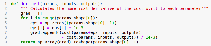
and similarly for the derivatives w.r.t $t_k$. Now, coding this up for your numerical simulations can be arduous. But one might argue that we can go by approximating the derivatives, rather than obsessing about analytically calculating them. This brings me to the second alternative: derivatives using finite differences. Let’s write a simple function to calculate derivatives for \ref{decomp} (which might change a bit for different cost functions, parameterizations, and the shape of the parameter arrays being passed)

Well, in qgrad we can do just that, and that too analytically, in one line

from jax import grad
grad(cost)(params, ket_input, ket_output)

without worrying about what the analytic form of the derivative looks like and without needing to write a custom finite differences method.

This hopefully shows how qgrad can be handy for optimization tasks that involve Hamiltonian learning. With qgrad, one can perform circuit learning as well! A notebook on Variational Quantum Algorithms is already in works. To track the project on GitHub, open issues or pull requests, please follow this link.

References

1. Jing, Li, et al. “Tunable efficient unitary neural networks (eunn) and their application to rnns.” International Conference on Machine Learning. 2017.

2. Lloyd, Seth, and Reevu Maity. “Efficient implementation of unitary transformations.” arXiv preprint arXiv:1901.03431 (2019).

3. Kiani, Bobak Toussi, Seth Lloyd, and Reevu Maity. “Learning unitaries by gradient descent.” arXiv preprint arXiv:2001.11897 (2020).