Let me start by claiming that quantum machine learning is basically unitary learning. Take circuit learning for example. We start with an initial state, which is almost always $| 0 \rangle$, apply a bunch of gates in each layer and continue to do so based on how much is our appetite for decoherence goes. Then we knot qubits up with some entanglement and finally measure on some or all qubits with respect to an operator. We tune our gates until the rotation angles are just right to give us a close enough prediction compared to a fixed target state. The task here is to tune the angles of the parametrized gates just right to achieve the desired prediction. Now, each gate is essentially a unitary matrix. The circuit, which is nothing but a gigantic unitary generated by tensoring each of these gates together, is a huge unitary matrix that depends on being tuned with just the right parameters. Shall we call this unitary learning?

To establish the idea somewhat formally, we can define unitary learning as the task of learning an optimal parameter vector $\vec{\theta}_{opt}$ that parametrizes $U(\vec{\theta})$ such that $U(\vec{\theta})$ is close enough to some target unitary, $U$.

A natural question now is that what does $U(\vec{\theta})$ look like? Any parametrization that satisfies $U U^{\dagger} = I$ works. Commonly, parameterizations have an exponential term raised to some matrix (hamiltonian). For example, in Kwok Ho Wan et al. (2018) the authors use the following parametrization where the Paulis are raised in the exponential term

$$ \begin{equation}\label{unitary-decomp-oscar} U = \exp[i(\sum_{j_{1}….j_{N} = 0,…,0}^{3…3} \alpha_{j_{1}…j_{N}} (\sigma_{j_{1}} \otimes … \otimes \sigma_{j_{N}})] \end{equation} $$

where $\sigma_{i}$ for $i \in {1, 2, 3,}$ are Pauli matrices with $\sigma_{0}$ being $n \times n$ identity matrix, and $\alpha_{j_{1}…j_{N}}$ are the parameters to be tuned.

In another paper by Seth Lloyd and Reevu Maity, 2019, unitaries are parameterized like

$$ \begin{equation}\label{unitary-decomp-lloyd} U(\vec{t}, \vec{\tau}) = e^{-iB\tau_{N}}e^{-iAt_{N}} … e^{-iB\tau_{1}}e^{-iAt_{1}} \end{equation} $$

where $\vec{t}$ and $\vec{\tau}$ are parameter vectors, each of size $N$ and $A$ and $B$ are chosen from the Gaussian Unitary Ensemble such that they generate the entire Lie algebra of $SU(d)$, where $d$ is the dimension of the unitary, $U(\vec{t}, \vec{\tau})$. I state this fact for completeness and we shall not refer to it again in the blog, so don’t worry if it sounds recondite.

Equations \ref{unitary-decomp-oscar} and \ref{unitary-decomp-lloyd} are just two examples of parameterization schemes of a unitary matrix, and as I said, there can be many. But here’s the question. What if I want to take a derivative of this unitary for some, say, learning task. Let’s say we follow the parametrization \ref{unitary-decomp-lloyd} for this. Although one can analytically write out the derivative as

$$ \begin{equation}\label{der-unitary-decomp-lloyd} \frac{\partial U(\vec{t}, \vec{\tau})}{\partial t_{k}} = e^{-iB\tau_{N}}e^{-iAt_{N}} … e^{-iB\tau_{k}}(-iA)e^{-iAt_{k}} … e^{-iB\tau_{1}}e^{-iAt_{1}} \end{equation} $$

(and similarly for $\frac{\partial U(\vec{t}, \vec{\tau})}{\partial \tau_{k}}$), it would be nice to be able to autodifferentiate these functions while doing numerical experiments. There are several different parameterizations and writing the code to calculate the derivative each time you change the parametrization scheme can be arduous.

If you have been reading my blog, you might know that my GSoC project involves using JAX to bring autodiff capabilities to quantum routines, so you know now where this is going. If we try to take such derivatives using JAX, it complains. JAX does not support the autodifferentiation (actually, it does support forward diff now, but backward diff is still a work in progress) of functions that have a matrix as a power of the exponential function. If you write something as simple as

import jax.numpy as jnp

def exp_mat(A):
    return jnp.sum(expm(A))

grad(exp_mat)(jnp.eye(2))

JAX throws

ValueError: Reverse-mode differentiation does not work for lax.while_loop or lax.fori_loop. Try using lax.scan instead.

While JAX developers are at it, my GSoC mentor Shahnawaz Ahmed suggested an alternate way to parametrize unitaries that does not involve matrices in exponential powers. This parametrization is detailed in C. Jarlskog, 2005.

$$ \begin{equation}\label{no-exp-unitary-decomp} X^{(n)}=\Phi^{(n)}(\vec{\alpha}) V^{(n)} \Phi^{(n)}(\vec{\beta}) \end{equation} $$ where matrices $\Phi$ are diagonal unitary matrices. $\Phi^{(n)}(\vec{\alpha})$ is defined as $$ \begin{equation} \Phi^{(n)}(\vec{\alpha}) = \begin{pmatrix} e^{i \alpha_{1}} & & & & \\ & e^{i \alpha_{2}} & & \\ & & \bullet & &\\ & & & \bullet &\\ & & & & e^{i \alpha_{n}} \end{pmatrix} \end{equation} $$

and $\Phi^{(n)}(\vec{\beta})$ is similarly defined with $\alpha$ entries replaced with $\beta$ entries, where $\alpha$’s and $\beta$’s are real. Wait, didn’t we want to avoid things in the power of exponents? Because if that was the goal, then \ref{no-exp-unitary-decomp} certainly does not achieve it. Well, the goal was to avoid matrices in powers of exponents (and that is what we achieve with \ref{no-exp-unitary-decomp}!). JAX is good with real (and even complex) numbers in the powers of exponents when it comes to autodiff. I, for example, recently reproduced Thomas Fösel et al.(2020.) with qgrad here. The paper has a cost function contribution via a SNAP gate that looks like

$$ \begin{equation}\label{snap-gate} \hat S(\vec{\theta}) = \sum_{0}^{n} e^{i \theta^{(n)}} |n\rangle \langle n| \end{equation} $$

Now here $\vec{\theta}$ consists of real numbers, not matrices that go to the power of the exponential. Sweet. Now, JAX wouldn’t complain. We then go on to smoothly reproduce the results of Thomas Fösel et al.(2020), where we start off from a vacuum state, $|0\rangle$ and apply three blocks of operators to lead to a target binomial state. Each block $\hat B$ looks like

$$ \begin{equation}\label{b-hat} \hat B = D(\alpha) \hat S(\vec \theta) D(\alpha)^{\dagger} \end{equation} $$

Here $D(\alpha)$ is the displacement operator (that comes with qgrad) with displacement $\alpha$ and $\hat S(\vec \theta)$ is the SNAP gate with parameter vector $\vec(\theta)$ of length $N$, the size of the Hilbert space.

Pause here for a bit. You (an astute reader?) might have noticed that if matrices are not allowed in exponentials, then how do we deal with the Displace operator, $D(\alpha)$, in \ref{b-hat} because it has creation and annihilation operators in the power of the exponent. A fellow GSoC student, Jake Lishman, suggested a scheme that uses eigendecomposition to avoid this problem. See the discussion here and the code here.

Okay, back to binomial state learning. The particular binomial state that the Thomas Fösel et al. learn from a vacuum state is

$$ \begin{equation}\label{binomial-state} b_{1} = \frac{\sqrt 3 |3\rangle + |9\rangle}{2} \end{equation} $$

The visual below shows the learning trajectory along various points during the learning routine, where each row represents the Hinton and Wigner plots at almost equally separted times during the learning schedule, starting from the first row (vacuum state):

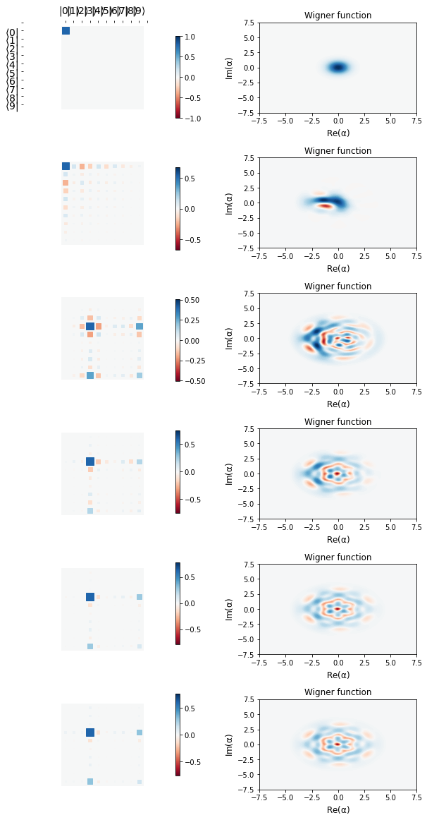
We see that the last row above (apart from being beautiful) is very close to the target binomial state, $b_{1}$ below

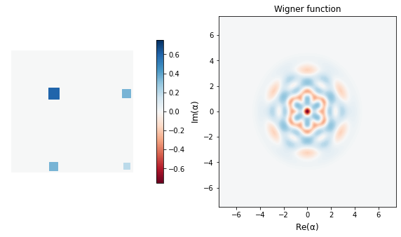
One can run a greater number of epochs for even better learning (that is to remove those little orange traces in the Hinton plot). But you get the idea. Without qgrad, one would need to write custom functions for the number states, dagger operator, etc, and figure out the trick for the Displace operator (without the matrix exponential). qgrad brings all of this together packaged for the user. This is just the beginning. We are exploring what we can do with qgrad, and we are excited to see what you will do in about a month’s time when we will release the first version of this package.

As to why did I talk about unitary parameterizations? Well, the objective was to show what we can’t do with JAX and how we can go about it (as we did with the Displace operator). The goal now is to is to construct arbitrary unitary matrices, following a scheme like \ref{no-exp-unitary-decomp} without matrix exponentials, much like what we did for Displace. By the way, if you know of other related unitary parameterizations that do not involve matrix exponentials, free to drop your suggestions in the comments below!

Once I am done writing the autodifferentiable unitary parametrization, I shall make (hopefully a better organized) post about unitary learning, where I explain from ground-up, what unitary learning is, implement it without qgrad, and then implement it with qgrad to juxtapose how qgrad would emancipate you from the shackles of writing gradient functions for cost functions involving expoentiating a hamiltonian. Because in autodiff, we trust!

References

1. Kwok Ho Wan, Feiyang Liu, Oscar Dahlsten, M.S.Kim. Learning Simon’s quantum algorithm. https://arxiv.org/abs/1806.10448 (2019).

2. Seth Lloyd, Reevu Maity. Efficient implementation of unitary transformations. https://arxiv.org/abs/1901.03431 (2019).

3. C. Jarlskog. A recursive parametrization of unitary matrices. https://aip.scitation.org/doi/full/10.1063/1.2038607 (2005).

4. Thomas Fösel, Stefan Krastanov, Florian Marquardt, Liang Jiang. Efficient cavity control with SNAP gates. https://arxiv.org/abs/2004.14256 (2020).