Disclaimer: This blog essentially summarizes this amazing review paper: Automatic Differentiation in Machine Learning: a Survey. All the tables and (fancy) images in the blog are taken from the paper. Invested readers should check out the full paper (linked).

Autodiff (short for Autodifferentiation) is extensively used in modern machine learning tasks. Libraries like Tensorflow, Pytorch, JAX and several others have made it easier to calculate the derivatives of arbitrary functions. In this blog, I will be going through the theory behind autodiff, explain what autodiff is NOT, and finally chain it up to machine learning (with a small code-snippet too).

Although I just promised to link machine learning later, the following example serves as a good motivation to start out with autodiff. Suppose that we want to perform backpropagation on a neural network that looks like this.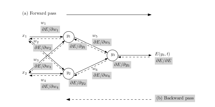

Image Source: Automatic Differentiation in Machine Learning: a Survey

Now, in order to do backprop, we need to take derivatives with respect to every weight in the network. In the worst case, for fully connected networks, this scales at least with the number of connections in the network. This, at first, seems like a daunting task since we have to take as many derivatives as there are connections in our network, and that too with respect to different parameters. Here is where the motivation for autograd comes in. We can calculate the derivatives with respect to all the weight parameters in just one backward pass. We shall do an example later in the blog to see for ourselves.

To further motivate the idea of autodiff, we shall see what are the shortcomings of some other derivative techniques, and how autodiff chimes in with a better solution.

Derivatives by Finite Differences

A widely used technique for approximating the derivatives is the finite differences method. One can understand this technique from the first principles. What is the small change in my function, $f$, corresponding to a small change in the value of the function parameter ($x$ in this case). For a single-valued function, the so-called forward difference method

approximates the derivative with a truncation term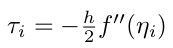

The derivates can be better approximated, with $\tau_{i} = O(h^2)$, using the centered-difference approximation, but again that would only be an approximation. Secondly, if you are familiar with Numerical Analysis, you must know that with numerical methods like these, we are faced with issues of consistency, convergence, and stability of the numerical solution. For our purposes, however, it should suffice to keep in mind that these methods only approximate the derivative. Ideally, we would want the exact derivative – and autodiff gives us just that!

Symbolic Differentiation

Another technique that is employed by softwares like MATLAB and Mathematica is called symbolic differentiation. The good thing about symbolic differentiation is that it gives exact derivatives. However, it has its failings. Firstly, for non-elementary functions, it might need the derivative to be hand-calculated. Even worse, when your functions become increasingly complex, a phenomenon called expression swell occurs. Authors of the review paper cite a very compelling example in the following table:

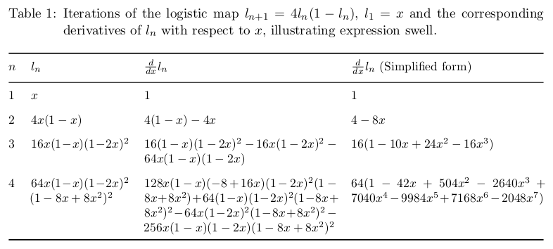
Image Source: Automatic Differentiation in Machine Learning: a Survey

Divide and Differentiate!

What autodiff does is to essentially deal with both the shortcomings of symbolic differentiation by using what I may call, a divide-and-differentiate strategy. As ‘autodifferentiators’, for any mathematical expression, we break it down into elementary operations whose derivatives are well-known (no more hand-calculating non-elementary derivatives), store those derivatives as intermediate variables (no more expression swell), and then use those derivatives in the chain rule to get the desired derivative. In order to better visualize the dependencies among these variables, it is a standard practice to make a computational graph of the function, $f(x_{1}, x_{2},…,{x_{n}})$. Let’s consider a concrete example of a two-variable function here

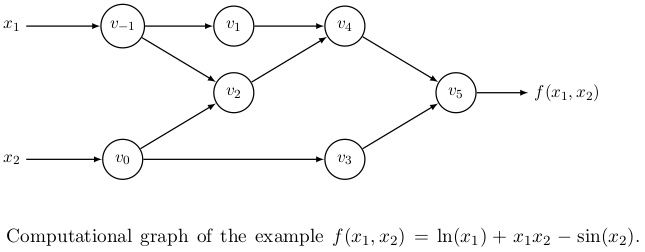Image Source: Automatic Differentiation in Machine Learning: a Survey

The intermediate nodes in the computational graph above represent the intermediate variables that in turn represent our elementary intermediate computations (fret not, you will see what operations these intermediate nodes represent in the forward mode example below). Actually, such computational graphs are what Pytorch makes for you under the hood. It makes something called a dynamic computational graph, where the user defines a model and the computational graph is constructed with the forward computation on the fly. On the other hand, static computational graphs like those in Theano, are constructed based off of the model before execution. Theano-type graphs remain fixed, hence static, while different data values are plugged in. Note that the terms static and dynamic refer to the graph topology and not to the data flow architectures.

Back to autodiff. In order to take the desired functional derivative with respect to any of the function parameters, we would be needing to calculate the intermediate derivatives as well.

For notational convenience, let’s define,

Forward Mode Autodiff

The first example we shall consider is of something called forward mode autodiff. In forward mode autodiff, we start from the left-most node and move forward along to the right-most node in the computational graph – a forward pass. This table from the survey paper succinctly summarizes what happens in one forward pass of forward mode autodiff.

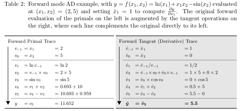Image Source: Automatic Differentiation in Machine Learning: a Survey

Note that the initializations in the first block of the derivative trace column above form a unit vector (if put together as a column vector). And that is not a coincidence. The variable with respect to which the derivative is being calculated is $1$ and others are $0$ in this initialization routine. The rest, as I said before, involves calculating elementary derivatives using the expressions in the left column and leveraging the chain rule to obtain the intermediate derivatives at each step. Finally, we obtain the desired derivative with respect to the first variable, $x_1$. To calculate $\frac{\partial y}{\partial x_{2}}$, we would have to perform another forward pass. Generally, for functions

we just need one forward pass. However, in the worst case, where the function input resides in an $n-$dimensional input space,

we would need $n$ forward passes to calculate all the desired derivatives – one derivative with respect to each of the $n$ input parameters.

Reverse Mode Autodiff

With forward mode autodiff under our belt, we can naturally guess the second type of autodifferentiation: reverse mode autodiff. Unlike the forward mode, the derivatives here are calculated in reverse, from the outputs to the inputs (right to left). But in order to go from the outputs back to the inputs, we need to reach the outputs beginning from the inputs to begin with (that was a bit of a mouthful, sorry). Now, this necessitates the forward pass on the graph to calculate just the forward primal trace (not the derivatives) like the left column in Table 2. And then we begin calculating the derivatives, starting from the outer-most node. A bit more notation here. We represent the intermediate derivatives here by

In the case of backprop, $y$ would be the error value as shown in the first figure. In fact, it would be helpful to keep backprop in mind while we solve the upcoming example for reverse mode autodiff. Making an analogy with backprop, suppose that we are interested in calculating the error derivative with respect to a particular weight. The minor difference in our case is that we are not dealing with network weights in our example. Well, there is no network, to begin with. We have inputs instead. So, in our case, we desire to calculate the derivatives $\frac{\partial y}{\partial v_{-1}}$ and $\frac{\partial y}{\partial v_{0}}$ of the output node with respect to the input parameters, $v_{-1}$ and $v_{0}$. Now, to do that, we would need to employ the chain rule. In order to, say, calculate $\frac{\partial y}{\partial v_{-1}}$, we would need to calculate

$$\frac{\partial y}{\partial v_{-1}} = \frac{\partial y}{\partial v_{1}}\frac{\partial v_{1}}{\partial v_{-1}} + \frac{\partial y}{\partial v_{2}}\frac{\partial v_{2}}{\partial v_{-1}}$$

since $v_{-1}$ is only directly connected to $v_{1}$ and $v_{2}$ in the computational graph. This Table from the survey paper, again, lucidly summarizes the calculations for reverse mode autodiff for the same example.

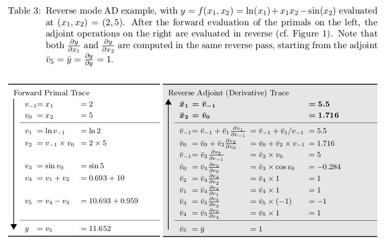
Image Source: Automatic Differentiation in Machine Learning: a Survey

Here is where things get interesting. Note that both $\frac{\partial y}{\partial x_{1}}$ and $\frac{\partial y}{\partial x_{0}}$ are evaluated in the same reverse pass. This is an improvement over the forward mode autodiff, where we saw that in the worst case when $f : \mathbb{R^{n}} \rightarrow \mathbb{R} $, forward mode autodiff needed $n$ passes. However, for reverse mode autodiff, such a function shall only need $one$ pass (but at the cost of increased storage requirements of all the intermediate variables). Since many machine learning tasks, like the training of deep neural networks, involve calculating the derivatives of the cost function that depends on a plethora of parameters in the feature space, reverse mode autodiff naturally arises to be the winner for such machine learning tasks. Really, backprop is just a special case of reverse mode autodiff applied to the network’s cost function.

Implementation

This quote is overused in tech blogs to the point that it almost seems banal. But let me just use it one more time (pls?)

Talk is cheap. Show me the code.

– Linus Torvalds

Since the core developers of the famed Autograd library have now moved over to actively develop JAX instead, we might as well just start with JAX.

import jax.numpy as np
from jax import grad

def f(x1,x2):
    """Returns the value of the function used in previous examples"""
    return np.log(x1) + x1*x2 - np.sin(x2)

#grad returns the gradient vector 
grad_f1 =  grad(f, argnums=0) #derivative wrt x1
grad_f2 =  grad(f, argnums=1) #derivative wrt x2

print(grad_f1(2.0,5.0))
# 5.5

print(grad_f2((2.0,5.0))
# 1.7163378

print(grad(grad(f))(2.0,5.0)) #second order derivative wrt x1
# -0.25

Verified! Our calculated values $5.5$ and $1.716$ (Table 3) of $\frac{\partial y}{\partial x_{1}}$ and $\frac{\partial y}{\partial x_{2}}$ respectively reconcile with what JAX gives us.

Autodiff has been around since the 1970s, but the machine learning community somehow did not take note. I should say that Autodiff and machine learning communities were two separate fields of research until recently (and still are). Both fields, however, have gained from one another, and there’s still a long way to go.